1 Introduction to AI and Big Data
Artificial intelligence (AI) has seen remarkable progress in recent years, transforming from a specialized field into everyday technology that millions of people now use for writing, coding, and problem-solving. These advances have been fueled by machine learning (ML) methods with a wide variety of applications, including:
- Computer vision (e.g., image recognition, autonomous vehicles),
- Natural language processing (e.g., chatbots, translation, sentiment analysis),
- Speech recognition (e.g., voice assistants),
- Recommendation systems (e.g., Netflix, Amazon, Spotify),
and many more. These tools also have many potential applications in economics and finance and can be invaluable for extracting information from the ever-growing amounts of data available. As current (or future) Banco de España employees, you are in a unique position to work with large datasets that are often not available to the general public. This presents a unique opportunity to apply these methods to a wide range of problems.
While the field can be technical, barriers to entry are not as high as they may seem. Modern programming languages like Python, combined with powerful open-source libraries (e.g., scikit-learn, PyTorch), have made machine learning accessible to practitioners without requiring a deep background in mathematics or computer science. This course aims to provide you with the foundational knowledge and practical tools to apply machine learning methods to problems in economics and finance.
1.1 How is AI Relevant for You?
You might have heard of some well-known advances in AI from recent years:
- Conversational AI: ChatGPT, Claude, and Gemini respond to complex prompts and reason through multi-step problems
- Image generation: Midjourney, DALL-E 3, and Stable Diffusion create photorealistic images from text descriptions
- Code assistants: GitHub Copilot and Claude Code help programmers generate and edit code
- Video generation: Sora and Veo produce videos from text prompts
These are just a few examples of consumer-facing AI applications.
While these examples are impressive and can be very useful in various contexts. There is a wide range of potential applications that might be relevant for your work which go beyond these examples. For example, machine learning methods have been used in practice to
- Predict loan or firm defaults based on financial statements and alternative data,
- Detect fraud patterns in real-time transaction data,
- Automate document processing and information extraction from regulatory filings,
- Monitor news and social media for early warning signals, or
- Forecast macroeconomic indicators and stress test scenarios
to just name a few examples. Bank for International Settlements (2021) and Bank for International Settlements (2025) provide an overview of how machine learning methods have been used at central banks in recent years.
To give you a few more ideas from academic research, machine learning techniques have been used to, for example,
- Detect emotions in voices during press conferences after FOMC meetings (Gorodnichenko et al. 2023),
- Identify Monetary Policy Shocks using Natural Language Processing (Aruoba and Drechsel 2022),
- Solve macroeconomic models with heterogeneous agents (Maliar et al. 2021; Fernández-Villaverde et al. 2023, 2024; Kase et al. 2022), or
- Estimate structural models with the help of neural networks (Kaji et al. 2023).
Varian (2014), Athey and Imbens (2019), Korinek (2023), and Dell (2025) provide further examples and discuss how these methods complement traditional econometrics.
Before diving into specific techniques, let’s clarify some terminology and understand where machine learning fits within the broader field of artificial intelligence.
1.2 Overview of Artificial Intelligence
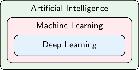
Artificial intelligence (AI), machine learning (ML), and deep learning (DL) are often used interchangeably in the media. However, they describe more narrow subfields (Microsoft 2024):
- Artificial Intelligence (AI): Any method allowing computers to imitate human behavior.
- Machine Learning (ML): A subset of AI including methods that allow machines to improve at tasks with experience.
- Deep Learning (DL): A subset of ML using neural networks with many layers allowing machines to learn how to perform tasks.
More recently, with the rise of large language models (LLMs) such as ChatGPT, several new terms have become popular:
- Generative AI refers to models that create new content—text, images, music, or video based on patterns learned from training data. ChatGPT and Midjourney are examples of generative AI.
- Predictive AI refers to models used to make predictions or classifications based on input data, such as predicting loan defaults or classifying images.
- Agentic AI refers to systems that can autonomously plan and execute multi-step tasks, use external tools, and take actions in the real world with minimal human oversight. Examples include AI coding assistants that can browse documentation, run tests, and edit files, or AI agents that can book travel or manage emails.
You may also encounter the term Artificial General Intelligence (AGI), which refers to hypothetical systems capable of human-level reasoning across a wide range of tasks. Unlike current AI, which excels at specific tasks, AGI would generalize to novel problems without task-specific training. While AGI is a topic of active research and debate, no consensus exists on how close we are to achieving it or even how to define it precisely.1 AGI and related concepts are beyond the scope of this course.
1.3 What is Machine Learning?
In this course, we will be mainly concerned with the subfield of artificial intelligence known as machine learning.
1.3.1 Definition
Murphy (2012) provides a simple definition of machine learning as
[…] a set of methods that can automatically detect patterns in data, and then use the uncovered patterns to predict future data, or to perform other kinds of decision making under uncertainty […]
Therefore, machine learning provides a range of methods for data analysis. In that sense, it is similar to statistics or econometrics.
A popular, albeit more technical, definition of ML is due to Mitchell (1997):
A computer program is said to learn from experience \(E\) with respect to some class of tasks \(T\), and performance measure \(P\), if its performance at tasks in \(T\), as measured by \(P\), improves with experience \(E\).
In the context of this course, experience \(E\) is given by a dataset that we feed into a machine-learning algorithm, tasks \(T\) are usually some form of prediction that we would like to perform (e.g., loan default prediction), and the performance measure \(P\) is the measure assessing the accuracy of our predictions.
1.3.2 Relation of Machine Learning to Statistics and Econometrics
We have already mentioned that machine learning is similar to statistics and econometrics, in the sense that it provides a set of methods for data analysis. The focus of machine learning is more on prediction rather than causality meaning that in machine learning we are often interested in whether we can predict A given B rather than whether B truly causes A. For example, we could probably predict the sale of sunburn lotion on a day given the sales of ice cream on the previous day. However, this does not mean that ice cream sales cause sunburn lotion sales, it is just that the sunny weather on the first day causes both.
Varian (2014) provides another example showing the difference between prediction and causality:
A classic example: there are often more police in precincts with high crime, but that does not imply that increasing the number of police in a precinct would increase crime. […] If our data were generated by policymakers who assigned police to areas with high crime, then the observed relationship between police and crime rates could be highly predictive for the historical data but not useful in predicting the causal impact of explicitly assigning additional police to a precinct.
Nevertheless, leaving problems aside where we are interested in causality, there is still a very large range of problems where we are interested in mere prediction, such as loan default prediction, or credit card fraud detection.
1.4 The Role of Big Data
The term big data refers to datasets that are too large or complex to be processed by traditional data processing methods. While there is no strict definition and the term is often used as a buzzword or marketing term, big data is often characterized by the “three Vs” (Laney 2001):
- Volume: The sheer amount of data generated and stored.
- Velocity: The speed at which new data is generated and needs to be processed.
- Variety: The different types of data (structured, unstructured, semi-structured) from various sources.
In the context of banking and finance, big data sources include:
- Transaction records (credit cards, payments, transfers)
- Customer interactions (call centers, online banking, mobile apps)
- Market data (stock prices, exchange rates, trading volumes)
- Alternative data (social media sentiment, satellite imagery, web scraping)
- Regulatory filings and reports
The combination of big data and machine learning creates a powerful synergy: machine learning algorithms thrive on large datasets, as more data generally leads to better pattern recognition and more accurate predictions. Conversely, traditional statistical methods often struggle with the high dimensionality and complexity of big data, making machine learning approaches increasingly attractive.
In this course, we will focus on machine learning methods that can, in principle, handle large datasets effectively. However, due to time constraints and the difficulty of the involved topics, we will put less emphasis on other important big data aspects such as distributed computing or data engineering. Varian (2014) provides a brief overview of big data and
1.5 History of Artificial Intelligence
Early contributions to the field reach back at least to McCulloch and Pitts (1943) and Rosenblatt (1958). They attempted to find mathematical representations of information processing in biological systems (Bishop 2006). As pointed out by Schmidhuber (2022), even earlier contributions in the form of linear regression2 go back to work from Adrien-Marie Legendre and Johann Carl Friedrich Gauss around 1800, while some of the mathematical tools at the heart of today’s AI models are even older than that. The term “artificial intelligence”, however, is much more recent and was coined only in 1956 at a conference at Dartmouth College (Schmidhuber 2022).
1.5.1 Broad Developments in AI
Given the long history of AI, I will only show some broad developments in the field since the 1950s:
- 1950s-60s: Early work on neural networks (e.g., perceptron by Rosenblatt (1958)) similar to what is used in deep learning today.
- 1970s-80s: Development of expert systems (e.g., MYCIN). These are computer programs that mimic the decision-making abilities of a human expert in a specific domain. They use a set of rules and knowledge bases to make decisions and solve problems.
- 1990s-2000s: Shift towards a more data-driven approach with statistical methods and machine learning (e.g., support vector machines, decision trees, etc.)
- 2010s: Deep learning revolution (e.g., successful application of neural networks in many domains such as computer vision, natural language processing, etc.)
- 2020s: Rise of large language models (e.g., GPT-3, ChatGPT) and generative AI (e.g., DALL-E, Midjourney)
1.5.2 Why has AI Become So Popular Recently?
The field has grown substantially mainly in recent years due to
- Advances in computational power of personal computers
- Increased availability of large datasets \(\rightarrow\) “big data”
- Improvements in algorithms
Figure 1.2 shows how the number of transistors on a microchip has increased over time. This increase in computational power has allowed for more complex machine learning algorithms to be run on personal computers. This trend is often referred to as Moore’s Law which states that the number of transistors on a microchip doubles approximately every two years. While the trend has slowed down in recent years, the increase in computational power has been a key driver for the recent advances in AI.
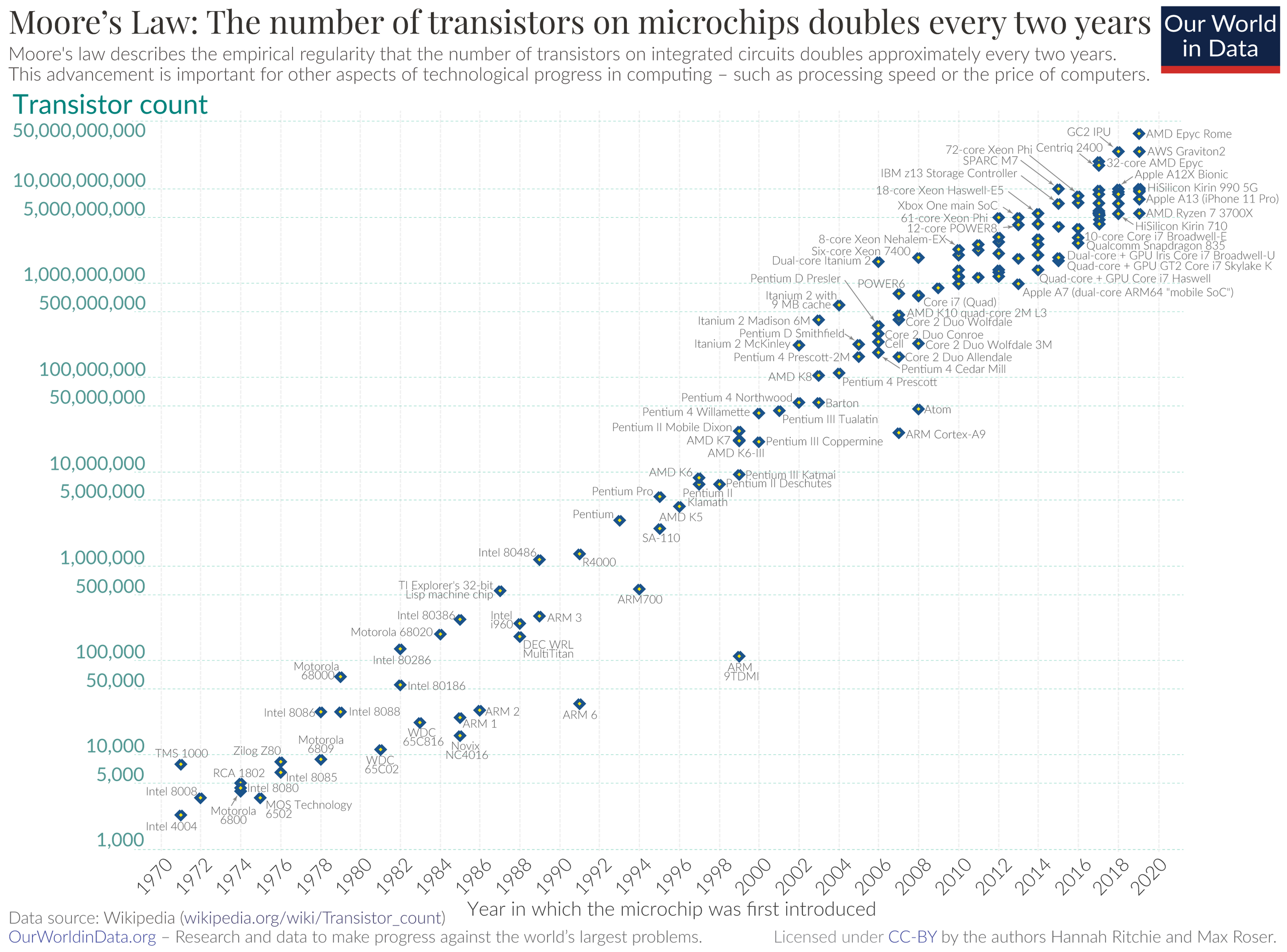
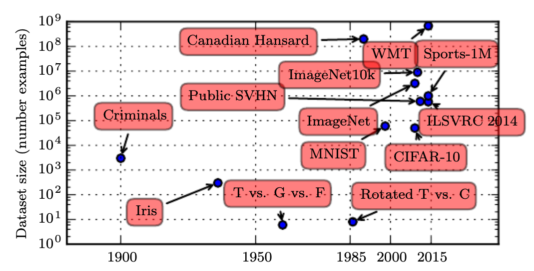
Figure 1.3 shows how the size of popular datasets in machine learning has increased over time. Larger datasets allow machine learning algorithms to learn more complex patterns in the data which often leads to better performance. Note that the figure is in log scale meaning that for each tick on the y-axis, the dataset size increases by a factor of 10. Unfortunately, the figure ends in 2015 and dataset sizes have continued to grow since then. For example, GPT-3 (released in 2020) was trained on a dataset with approximately 300 billion tokens (words or word pieces) (Brown et al. 2020). Even more recent models will have been trained on even larger datasets. Furthermore, as discussed in the section on big data, thanks to digitalization and the rise of the internet, some companies now have access to vast amounts of data on user behavior (e.g., Amazon has data on purchases made by its customers, Netflix has data on what movies users watch, etc.), which can be used to train machine learning models.
The need for large data sets still limits the applicability to certain fields. For example, in macroeconomic forecasting, we usually only have quarterly data for 40-50 years. Conventional time series methods (e.g., ARIMA) often still tend to perform better than ML methods (e.g., neural networks). However, in this particular case, with the advent of pretrained time series models, e.g., Chronos, this might change in the (near) future.
On the algorithmic side, there have been many improvements in optimization algorithm and model architectures (e.g., development of transformers) that have allowed for more efficient training of machine learning models. These improvements have also contributed to the recent advances in AI. Furthermore, a strong community effort has gone into open-sourcing machine learning frameworks (e.g., PyTorch) and pre-trained models (e.g., BERT, GPT) which has lowered the barrier to entry for many practitioners.
1.6 Types of Learning
Machine learning methods are commonly distinguished based on the tasks that we would like to perform, and the data that we have access to for learning how to perform said task. ML methods are commonly categorized into
- Supervised Learning: Learn function \(y=f(x)\) from data that you observe for \(x\) and \(y\)
- Unsupervised Learning: “Make sense” of observed data \(x\)
- Reinforcement Learning: Learn how to interact with the environment
Key for the distinction between supervised and unsupervised learning is whether we have access to labeled data (i.e., data where we observe both input features \(x\) and output labels \(y\)) or not, as the following example illustrates.
NoteExample: Fraud Detection
Suppose you work in a bank’s fraud detection department and want to identify fraudulent credit card transactions. The approach you take depends on what data you have available:
- Supervised Learning: If you have historical transaction data where each transaction is labeled as “fraudulent” or “legitimate” (e.g., from past investigations or customer reports), you can train a model to learn the patterns that distinguish fraud from normal transactions. The model learns a function that maps transaction features (amount, location, time, merchant type, etc.) to a fraud prediction. Once trained, the model can classify new, unseen transactions.
- Unsupervised Learning: If you don’t have labels, perhaps because fraud is rare and hard to identify, or you’re looking for new types of fraud that haven’t been seen before, you can use unsupervised learning to find unusual patterns. For example, a clustering algorithm might group transactions by similarity and flag transactions that don’t fit well into any cluster as potential anomalies worth investigating.
CautionTypes of Learning in Practice
Machine learning models might combine different types of learning. In the context of the previous example of fraud detection, one might use unsupervised methods to detect anomalies and flag suspicious transactions, followed by human review that generates labels, which then feed into supervised models for more accurate classification.
A related approach is semi-supervised learning, which uses a small amount of labeled data together with a large amount of unlabeled data. This is particularly useful when labeling is expensive or time-consuming—for example, having experts manually classify thousands of regulatory documents. The model learns patterns from the abundant unlabeled data while using the limited labels to guide its understanding.
Another example of combining different learning methods is provided by large language models (LLMs) such as ChatGPT. LLMs are typically trained using a combination of self-supervised learning (a form of unsupervised learning), supervised learning, and reinforcement learning.
The focus of this course will be on supervised learning. Nevertheless, let’s have a closer look at the three types of learning.
1.6.1 Supervised Learning
Supervised learning is probably the most common form of machine learning. In supervised learning, we have a training dataset consisting of input-output pairs \((x_n, y_n)\) for \(n=1,\ldots,N\). The goal is to learn a function \(f\) that maps inputs \(x\) to outputs \(y\).
The type of function \(f\) might be incredibly complex, e.g.
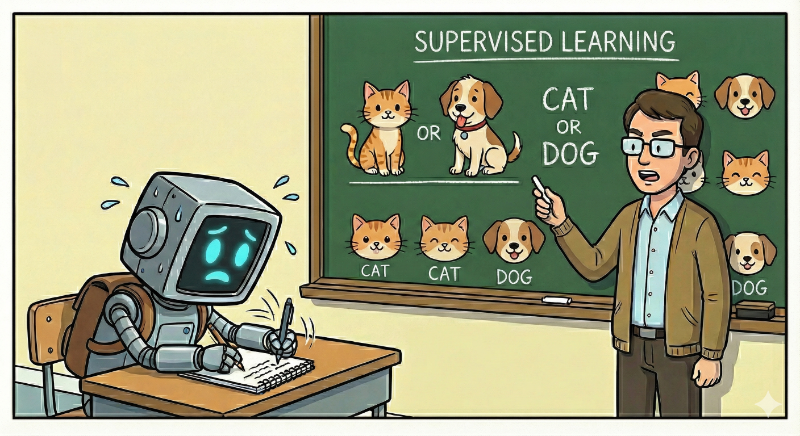
- From images of cats and dogs \(x\) to a classification of the image \(y\) (\(\rightarrow\) Figure 1.5)
- From text input \(x\) to some coherent text response \(y\) (\(\rightarrow\) ChatGPT)
- From text input \(x\) to a generated image \(y\) (\(\rightarrow\) Midjourney)
- From bank loan application form \(x\) to a loan decision \(y\)
Regarding terminology, note that sometimes
- Inputs \(x\) are called features, predictors, or covariates,
- Outputs \(y\) are called labels, targets, or responses.
Based on the type of output, we can distinguish between
- Classification: Output \(y\) is in a set of mutually exclusive labels (i.e., classes), i.e. \(\mathcal{Y}=\{1,2,3,\ldots,C\}\)
- Regression: Output \(y\) is a real-valued quantity, i.e. \(y\in\mathbb{R}\)
Let’s have a closer look at some examples of classification and regression tasks.
Classification
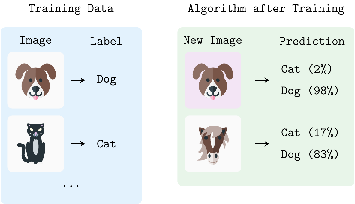
Figure 1.5 shows an example of a binary classification task. The algorithm is trained on a dataset of images of cats and dogs. The goal is to predict the label (i.e., “cat” or “dog”) of a new image (new in the sense that the images were not part of the training dataset). After training, the algorithm can predict the label of new images with a certain degree of accuracy. However, if you give the algorithm an image of, e.g., a horse it might mistakenly predict that it is a dog because the algorithm has never seen an image like that before and because it has been trained only for binary classification (it only knows two kinds of classes, “cats” and “dogs”). In this example, \(x\) would be an image in the training dataset and \(y\) would be the label of that image.
Extending the training dataset to also include images of horses with a corresponding label would turn the tasks into multiclass classification.
Regression
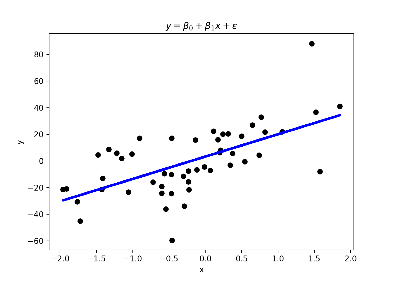
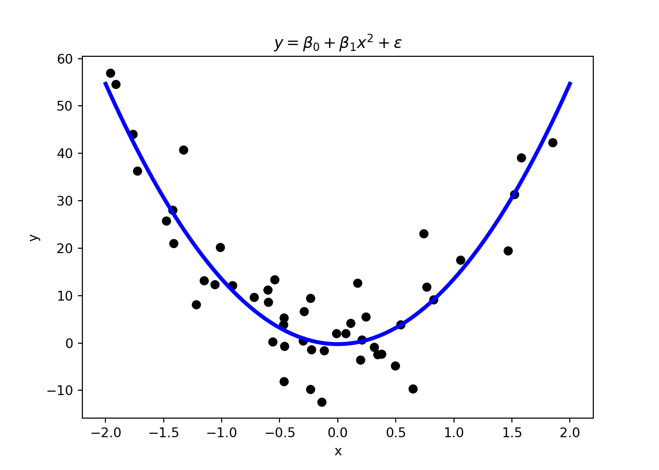
In regression tasks, the variable that we want to predict is continuous. Linear and polynomial regression in Figure 1.6 are a form of supervised learning. Thus, you are already familiar with some basic ML techniques from the statistics and econometrics courses.
Another common way to solve regression tasks is to use neural networks, which can learn highly non-linear relationships. In contrast to, for example, polynomial regression, neural networks can learn these relationships without the need to specify the functional form (i.e., whether it is quadratic as in Figure 1.6) of the relationship. This makes them very flexible and powerful tools. We will have a look at neural networks later on.
1.6.2 Unsupervised Learning
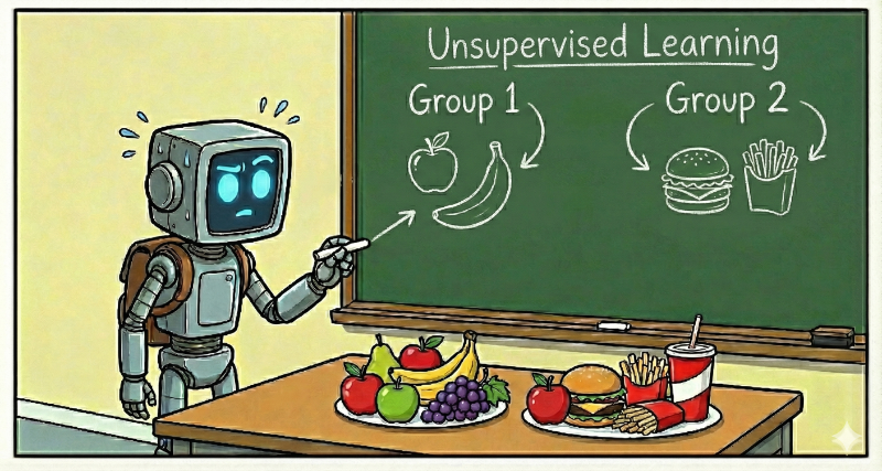
An issue with supervised learning is that we need labeled data which is often not available. Unsupervised learning is used to explore data and to find patterns that are not immediately obvious. For example, unsupervised learning could be used to find groups of customers with similar purchasing behavior in a dataset of customer transactions. Therefore, the task is to learn some structure in the data \(x\). Note that we only have features in the dataset and no labels, i.e., the training dataset consists of \(N\) data points \(x_n\).
Unsupervised learning tasks could be, for example,
- Finding clusters in the data, i.e. finding data points that are “similar” (\(\rightarrow\) clustering)
- Finding latent factors that capture the “essence” of the data (\(\rightarrow\) dimensionality reduction)
Let’s have a look at some examples of clustering and dimensionality reduction.
Clustering
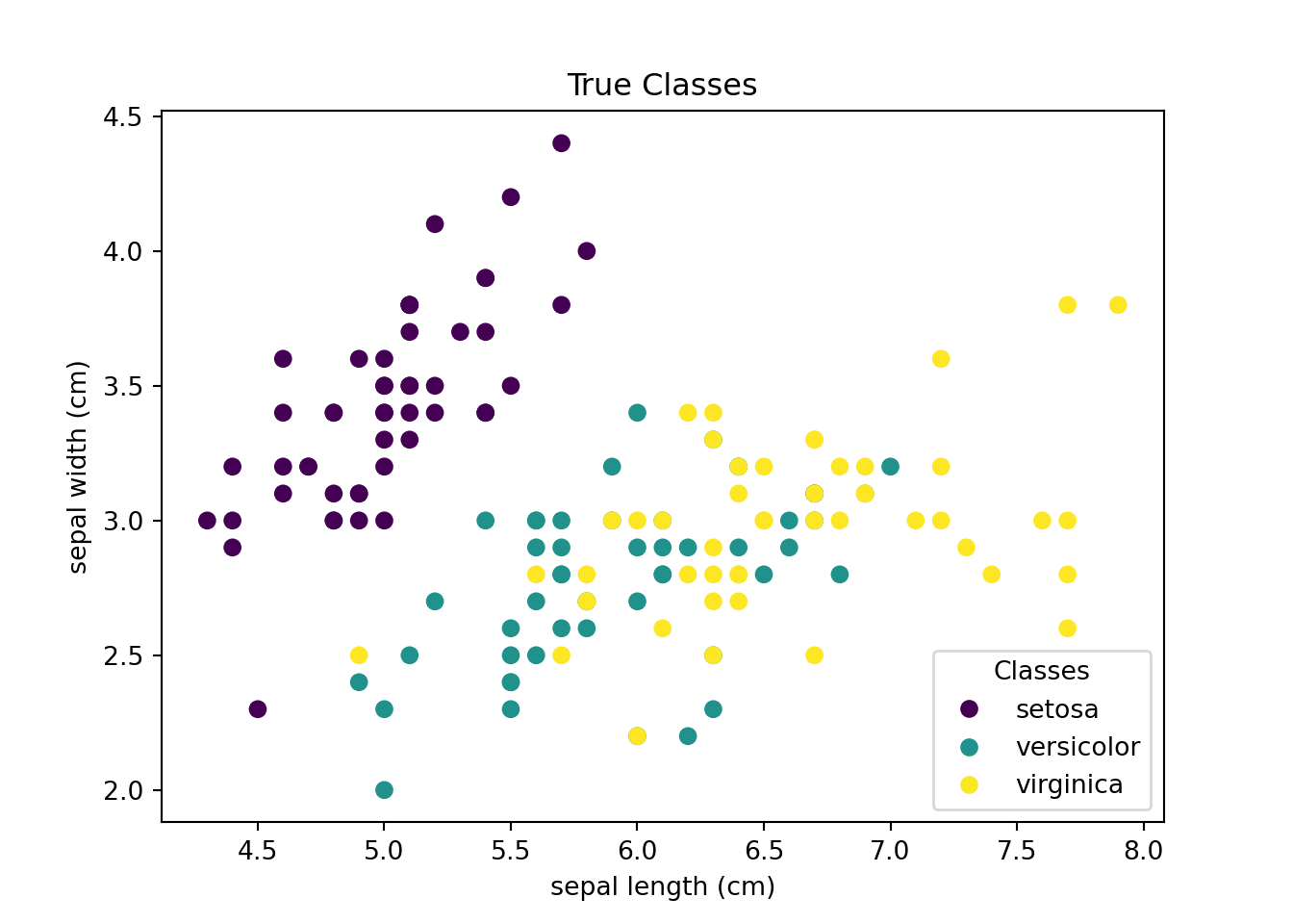
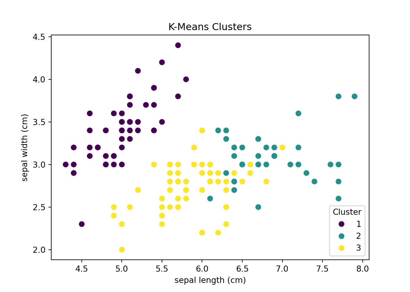
Clustering is a form of unsupervised learning where the goal is to group data points into so-called clusters based on their similarity. We want to find clusters in the data such that observations within a cluster are more similar to each other than to observations in other clusters.
Figure 1.8 shows an example of a clustering task. The dataset consists of measurements of sepal (and petal) length and width of three species of iris flowers. The goal is to find clusters based on just the similarity in sepal and petal lengths and widths without relying on information about the actual iris flower species. The left-hand panel of Figure 1.8, shows the actual classification of the iris flowers. The right-hand side shows the result of a k-means clustering algorithm that groups the data points into three clusters.

Dimensionality Reduction
Suppose you observe data on house prices and many variables describing each house. You might observe, e.g., property size, number of rooms, room sizes, proximity to the closest supermarket, and hundreds of variables more. A ML algorithm (e.g., principal component analysis or autoencoders) could find the unobserved factors that determine house prices. These factors sometimes (but not always) have an interpretation. For example, a factor driving house prices could be amenities. This factor could summarize variables such as proximity to the closest supermarket, number of nearby restaurants, etc. Ultimately, hundreds of explanatory variables in the data set might be represented by a small number of factors.
1.6.3 Reinforcement Learning
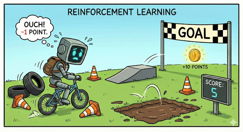
In reinforcement learning, an agent learns how to interact with its environment. The agent receives feedback in the form of rewards or penalties for its actions. The goal is to learn a policy that maximizes the total reward.
For example, a machine could learn to play chess using reinforcement learning
- Input \(x\) would be the current position (i.e., the position of pieces on the board)
- Action \(a\) would be the next move to make given the position
- One also needs to define a reward (e.g., winning the game at the end)
- Goal is then to find \(a=\pi(x)\) to maximize the reward
This is also the principle behind AlphaZero that learned how to play Go and chess.
Another example is MarI/O which learned how to play Super Mario World. The algorithm learns to play the game by receiving feedback in the form of rewards (e.g., points for collecting coins, penalties for dying) and then improves in playing the game by “an advanced form of trial and error”.
In this course, we will focus on supervised learning. However, we will look at some unsupervised learning techniques if time allows. Reinforcement learning is going beyond the scope of this course and will not be covered.
NoteMini-Exercise
Are the following tasks examples of supervised, unsupervised, or reinforcement learning?
- Predicting the price of a house based on its size and location (given a dataset of house prices and features).
- Finding groups of customers with similar purchasing behavior (given a dataset of customer transactions and customer characteristics).
- Detecting fraudulent credit card transactions (given a dataset of unlabeled credit card transactions).
- Detecting fraudulent credit card transactions (given a dataset of labeled credit card transactions).
- Recognizing handwritten digits in the MNIST dataset (see next section).
- Grouping news articles by topic based only on their content (without knowing the topics in advance).
- Predicting whether a customer will cancel their subscription next month, given historical data on customer behavior and cancellations.
- Classifying emails as spam or not spam, using a dataset where each email is labeled as spam or not.
- Training a robot to navigate a maze by receiving rewards for reaching the exit and penalties for hitting walls.
- Identifying unusual trading patterns in financial markets to flag potential market manipulation (given a dataset of trades with no labels indicating manipulation).
- Automatically categorizing incoming regulatory documents by topic (given a corpus of documents that have already been manually categorized).
- Training an agent to set interest rates in a simulated economy, receiving rewards based on how well it stabilizes inflation and output over time.
- Extracting the sentiment (hawkish vs. dovish) from central bank press releases (given a dataset of statements labeled by economists as hawkish or dovish).
- Reducing hundreds of macroeconomic indicators to a smaller set of latent factors that capture the state of the economy.
- Improving a chatbot’s responses by having users rate each reply as helpful or unhelpful after their conversation.
TipSolution
- Supervised learning (regression): We have labeled data (house prices) and want to predict a continuous value.
- Unsupervised learning (clustering): No labels; we’re finding structure in the data based on similarity.
- Unsupervised learning (anomaly detection): Without labels, we can only identify unusual patterns that deviate from normal behavior.
- Supervised learning (classification): With fraud/legitimate labels, we can train a classifier.
- Supervised learning (classification): MNIST includes digit labels (0–9) for each image.
- Unsupervised learning (clustering/topic modeling): No predefined topics; we discover them from the data.
- Supervised learning (classification): Historical cancellation data provides labels (churned/retained).
- Supervised learning (classification): Each email is labeled as spam or not spam.
- Reinforcement learning: The robot learns from rewards and penalties through interaction with its environment.
- Unsupervised learning (anomaly detection): No labels; we identify outliers that deviate from normal trading patterns.
- Supervised learning (classification): We have labeled categories and want to assign new documents to them.
- Reinforcement learning: The agent learns a policy through sequential interaction with the simulated economy, receiving rewards based on outcomes.
- Supervised learning (classification): Labeled sentiment data allows us to train a classifier.
- Unsupervised learning (dimensionality reduction): No labels; we’re finding latent structure (e.g., via PCA or factor models).
- Reinforcement learning (RLHF): The chatbot learns to generate better responses based on human feedback signals. This approach, known as Reinforcement Learning from Human Feedback (RLHF), is how models like ChatGPT are fine-tuned after initial training.
1.7 Popular Practice Datasets
There are many publicly available datasets that you can use to learn how to implement machine learning methods. Here are some well-known platforms with a large collection of datasets
- Kaggle,
- HuggingFace, and
- OpenML.
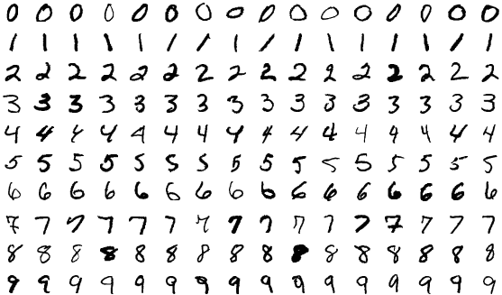
Another good source for practice datasets is the collection of datasets provided by scikit-learn. These datasets can be easily loaded into Python from the scikit-learn package. Furthermore, Murphy (2022) provides an overview of some well-known datasets that are often used in machine learning. For example, MNIST is a dataset of handwritten digits (see Figure 1.11) that is often used to test machine learning algorithms. The dataset consists of 60,000 training images and 10,000 test images. Each image is a 28x28 pixel image of a handwritten digit. The goal is to predict the digit in the image.
For more background, see Google Cloud’s overview of AGI.↩︎
As we will see this can be thought of as a basic form of an artificial neural network.↩︎